DynaSolver: Neural Operator for Autoregressive 4D Flow Prediction with Dynamic Boundaries

Video

Overview of RoboCFD-4D and DynaSolver (1:16).

Abstract

Neural operators provide efficient surrogates for computational fluid dynamics (CFD), but most are designed for static geometries and are not equipped to model unsteady flows induced by continuously moving boundaries. We study dynamic-boundary 4D CFD prediction for articulated moving geometries and introduce RoboCFD-4D, a temporally resolved robotic CFD benchmark spanning diverse morphologies and flow conditions. To address the computational and autoregressive challenges of this setting, we propose DynaSolver, a neural operator that explicitly conditions on boundary evolution and causal flow history. DynaSolver employs an efficient physical-token formulation that amortizes point-to-token projection across the operator stack, substantially reducing repeated point-space spatiotemporal computation while retaining accurate point-level reconstruction. We further introduce Replay-Augmented Parallel Training, which exposes the model to autoregressively generated histories while preserving parallel dense supervision, narrowing the gap between ground-truth-conditioned training and autoregressive rollout. Experiments on RoboCFD-4D show that DynaSolver achieves the best full-rollout accuracy among a broad range of learned CFD surrogates, with its advantage increasing as rollout proceeds, indicating substantially reduced autoregressive error accumulation.

Experiments

Quantitative comparison

On RoboCFD-4D Base we report relative L₂ (%) of velocity and pressure at selected rollout steps, plus full-rollout averages. Persistence is a no-learning baseline and is excluded from ranking. DynaSolver is not the strongest at the first step, but it is best from mid-horizon onward, so the full-rollout overall error is lowest.

Method	Per-frame Velocity ↓						Per-frame Pressure ↓						Avg. Vel. ↓	Avg. Pre. ↓	Overall ↓
Method	1	6	12	18	24	29	1	6	12	18	24	29	Avg. Vel. ↓	Avg. Pre. ↓	Overall ↓
GNOT	11.38	21.14	28.47	34.58	40.01	43.99	34.08	72.89	93.49	98.66	102.21	99.18	30.56	87.84	31.55
GAOT	14.46	19.54	23.58	26.93	29.66	31.19	40.96	57.70	66.52	75.18	84.08	90.67	24.60	70.25	25.32
CNO	9.32	19.36	24.27	28.49	35.25	47.04	34.24	77.09	87.29	98.14	108.89	120.71	27.12	91.52	28.28
P3D	9.32	17.07	22.62	26.70	30.44	32.36	32.55	62.66	76.03	85.25	96.86	102.08	23.72	78.82	24.61
MGN	9.49	19.70	23.69	25.88	27.66	28.55	29.32	65.02	79.25	86.55	96.78	99.86	23.48	79.44	24.51
DPOT	13.66	22.65	26.70	32.77	39.39	44.98	42.45	78.12	103.77	133.25	166.67	187.97	30.30	121.10	32.08
AB-UPT	14.75	19.60	23.36	25.68	27.92	29.38	42.29	77.47	91.30	96.30	97.54	96.23	23.83	86.84	25.03
UNO	11.71	18.17	22.82	26.91	34.53	62.31	34.13	58.36	71.43	81.76	104.69	156.99	27.32	81.55	28.40
U-Net	7.48	16.73	20.99	23.30	25.05	26.08	27.90	61.64	78.41	85.41	96.04	95.75	20.81	77.99	21.86
MSPT	9.28	19.15	23.18	25.89	28.14	29.94	27.70	61.18	73.90	86.65	101.71	110.88	23.42	79.14	24.39
Transformer_galerkin	11.89	19.49	23.07	28.43	35.67	42.74	38.61	69.13	96.66	115.08	136.97	168.67	26.86	104.64	28.11
DilResNet	8.55	17.99	22.08	23.90	25.04	25.30	29.00	61.87	78.00	83.80	86.84	84.99	21.44	74.56	22.30
PhysGTO	9.41	18.51	21.85	23.68	25.69	26.97	30.52	60.97	70.12	78.40	89.10	92.79	21.81	72.96	22.99
GNS	9.67	19.74	24.31	27.72	30.70	32.74	29.69	61.92	78.24	89.28	99.89	106.83	24.97	80.91	26.09
DeepONet	16.68	21.74	26.20	28.05	28.29	28.67	60.07	73.64	86.37	91.34	92.49	90.63	25.51	84.65	26.38
GraphViT	8.33	17.05	20.41	22.18	23.61	24.44	28.28	57.98	69.36	71.16	75.61	76.20	20.15	66.05	21.00
BSMS	8.44	17.30	21.20	24.12	26.66	28.85	27.01	54.20	61.57	68.21	77.84	81.24	21.78	63.92	22.51
FNO	10.70	18.04	22.07	26.54	33.95	42.81	31.13	52.02	60.85	66.83	71.30	76.06	25.49	61.69	26.08
LinearNO	10.26	16.81	19.74	21.66	22.92	23.84	29.14	52.05	60.81	65.82	72.07	72.55	19.82	61.00	20.58
MWT	9.55	16.50	18.67	20.26	22.03	23.35	32.05	57.19	70.58	83.28	97.58	106.52	18.97	76.64	20.11
Transolver	10.19	16.24	19.10	20.73	22.38	23.45	29.77	54.27	61.51	66.99	74.53	75.64	19.23	62.76	19.99
Persistence	14.14	20.78	19.80	20.42	20.92	21.35	40.17	60.19	54.16	54.63	58.75	58.21	20.14	56.09	20.95
DynaSolver (Ours)	11.61	16.27	17.37	17.86	18.06	18.36	34.02	53.19	57.48	59.17	60.37	61.61	17.07	56.35	17.71

Table 1. Quantitative comparison across rollout horizons on RoboCFD-4D Base. Best in green; second-best underlined. Persistence is not ranked.

Rollout error trends

The same Base evaluation as curves: overall, velocity, and pressure relative L₂ over the full autoregressive horizon. DynaSolver’s gap widens as rollout proceeds, especially for velocity, matching the late-horizon numbers in Table 1 (18.36% velocity and 61.61% pressure at step 29).

Overall

Velocity

Pressure

Figure 1. Rollout error evolution on RoboCFD-4D Base; curves are drawn frame by frame along the rollout horizon.

Accuracy versus training cost

Training cost versus overall rollout error

17.71%lowest overall error

−11.4%vs. next best, 19.99%

21learned baselines

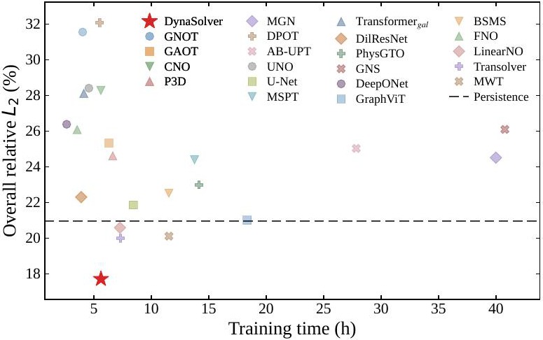
Each point is one learned surrogate, placed by its training time and full-rollout error on RoboCFD-4D Base. The dashed line marks Persistence, a no-learning baseline that copies the last state.

Most baselines trade one for the other: fast models stay near the Persistence line, while accurate ones need several times longer to train.

Two choices avoid this trade-off. The token-space operator skips repeated point-space work, and Replay-Augmented Parallel Training avoids slow sequential unrolling.

Figure 2. Training wall-clock versus overall rollout error on RoboCFD-4D Base.

Qualitative comparison

Thirty autoregressive rollout frames on three robots (A1, G1, and H1-2). The first panel is the ground-truth velocity field; the rest are point-wise velocity error of DynaSolver and five baselines. Click the board to pause or resume.

Robot

RoboCFD-4D Dataset

RoboCFD-4D is a temporally resolved CFD benchmark of articulated robots in motion. Below are twenty-two robots at u = 6 m/s and yaw 0°. Clips are muted loops; click a clip to pause it.

Method

1Efficient 4D Sequence Modeling

DynaSolver predicts the next velocity and pressure field from the robot geometry, its boundary motion, and a short causal history of flow states. It is designed to do this cheaply and with explicit temporal reasoning.

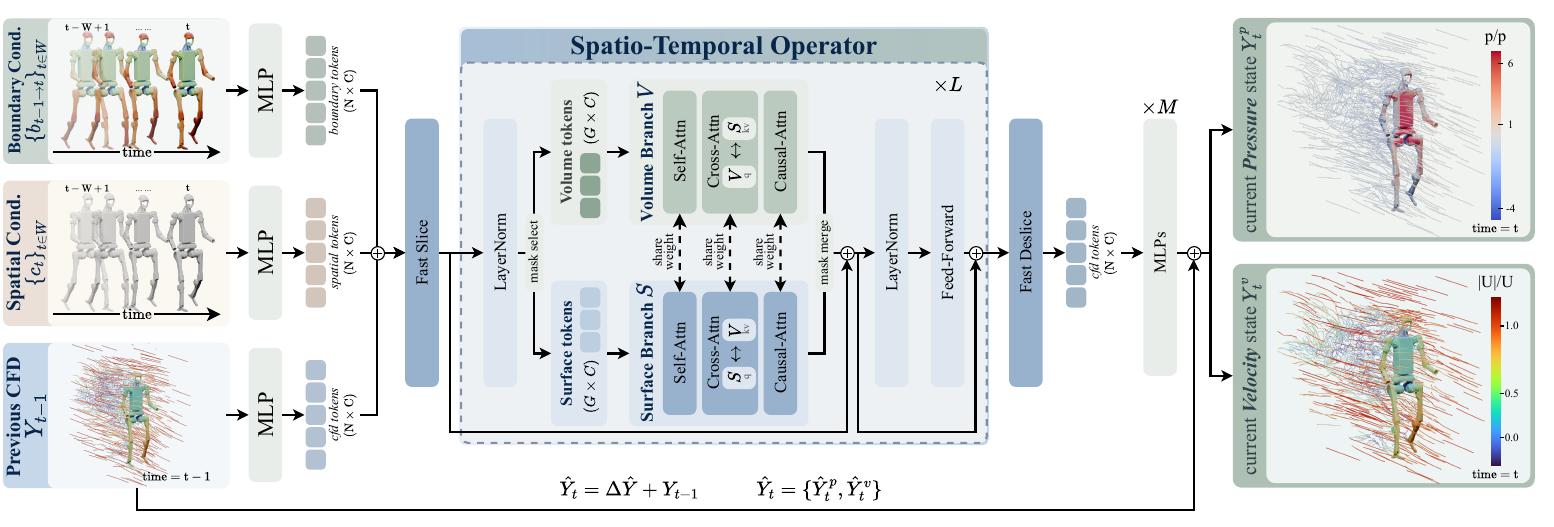
Figure 3. DynaSolver pipeline. A single Fast Slice / Fast Deslice pair encloses the whole spatio-temporal operator stack.

Efficiency

WhyEvery transition carries thousands of surface and volume points. Point-space operators re-project points to tokens and run point-wise feed-forward layers in every layer, so a temporal window multiplies this heavy cost by both depth and window length.

HowWe slice once: lifted point features are encoded into compact surface and volume physical tokens, all self-, cross-, causal attention and feed-forward layers operate in token space, and a single deslice with a light MLP decodes the point-wise residual field.

ResultFor a window of W transitions and L operator blocks, point–token projection runs O(W) rather than O(LW) times, so deeper temporal reasoning adds only token-space cost while outputs stay point-accurate.

Temporal modeling

1Boundary evolution injection. Each transition is conditioned on the boundary motion between adjacent frames, giving the operator explicit information on how the geometry moves instead of inferring it from the flow.

2Causal sliding window. A short history of up to W transitions supplies the memory that a single, partially observed flow state lacks; the window grows from the initial state and then slides forward.

3Causal temporal attention. A block-causal mask lets each transition aggregate information only from itself and earlier transitions, so the model reasons over history exactly as it will during rollout and predicts a residual on top of the previous state.

2Replay-Augmented Parallel Training

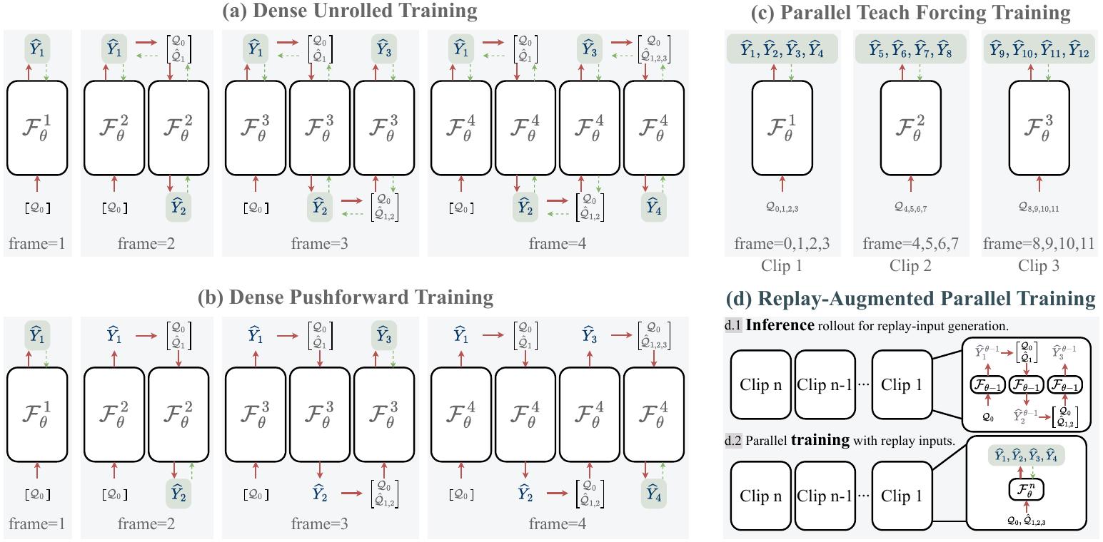
Figure 4. (a–b) sequential unroll and pushforward; (c) parallel teacher forcing; (d) our replay-augmented parallel training.

Training an autoregressive solver is a case of you can’t have your cake and eat it: fast training or robust rollout.

Unroll and Pushforward feed the model its own predictions, so rollout is robust, but they unroll sequentially and take about 16.5 h. Parallel teacher forcing supervises every transition in one block-causal pass (1.8 h), yet it only ever sees ground-truth histories, so the error grows to 18.18% once the model rolls out on its own outputs.

We close this train–inference gap without giving up parallelism. A frozen previous-epoch model rolls out replay histories without gradients, and the current model is trained on a mix of replay and clean clips in a single parallel pass with ground-truth targets.

Both at once: the lowest rollout error, 16.14%, in just 2.313 h, beating Unroll while training about 7.2× faster.

Training strategyOverall rollout L₂ (%)Training time (h)

RoboCFD-4D Mini, same DynaSolver architecture. Error bars start at 15%.

Citation

@misc{qian2026dynasolverneuraloperatorautoregressive,
  title         = {DynaSolver: A Neural Operator for Autoregressive 4D Flow Prediction with Dynamic Boundaries},
  author        = {Rui Qian and Shibo Dai and Mengjun Lin and Yuk-Kit Hou and Saining Zhang and Bohan Li and Junhao Chen and Hao Zhao and Chaojian Li},
  year          = {2026},
  eprint        = {2611.03595},
  archivePrefix = {arXiv},
  primaryClass  = {cs.LG},
  url           = {https://arxiv.org/abs/2611.03595},
}